32 KiB

Learn Foundational Math 3 by Building a Financial App
Each of these steps will lead you toward the Certification Project. Once you complete a step, click to expand the next step.
↓ Do this first ↓
Copy this notebook to your own account by clicking the File button at the top, and then click Save a copy in Drive. You will need to be logged in to Google. The file will be in a folder called "Colab Notebooks" in your Google Drive.
Step 0 - Acquire the Testing Library
Please run this code to get the library file from FreeCodeCamp. Each step will use this library to test your code. You do not need to edit anything; just run this code cell and wait a few seconds until it tells you to go on to the next step.
# You may need to run this cell at the beginning of each new session

!pip install requests

# This will just take a few seconds

import requests

# Get the library from GitHub
url = 'https://raw.githubusercontent.com/edatfreecodecamp/python-math/main/math-code-test-c.py'
r = requests.get(url)

# Save the library in a local working directory
with open('math_code_test_c.py', 'w') as f:
    f.write(r.text)

# Now you can import the library
import math_code_test_c as test

# This will tell you if the code works
test.step00()
Requirement already satisfied: requests in /usr/local/lib/python3.8/dist-packages (2.31.0)
Requirement already satisfied: charset-normalizer<4,>=2 in /usr/local/lib/python3.8/dist-packages (from requests) (3.2.0)
Requirement already satisfied: idna<4,>=2.5 in /usr/lib/python3/dist-packages (from requests) (2.8)
Requirement already satisfied: urllib3<3,>=1.21.1 in /usr/lib/python3/dist-packages (from requests) (1.25.8)
Requirement already satisfied: certifi>=2017.4.17 in /usr/lib/python3/dist-packages (from requests) (2019.11.28)
[33mWARNING: Running pip as the 'root' user can result in broken permissions and conflicting behaviour with the system package manager. It is recommended to use a virtual environment instead: https://pip.pypa.io/warnings/venv[0m[33m
[0m
[1m[[0m[34;49mnotice[0m[1;39;49m][0m[39;49m A new release of pip is available: [0m[31;49m23.1.2[0m[39;49m -> [0m[32;49m23.2.1[0m
[1m[[0m[34;49mnotice[0m[1;39;49m][0m[39;49m To update, run: [0m[32;49mpython3 -m pip install --upgrade pip[0m
Code test passed
Go on to the next step
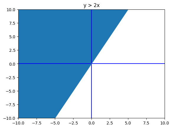
Step 1 - Graphing Inequalities
Learn Inequalities by Building Shaded Graphs. Notice how you set up the plot, like you learned in the last certification. Run the following code and you will see that the graph of y > 2x is not quite right. Because y is greater, the shading should be above the line. The second two arguments in the fill_between() function give a range of y values to shade. Change just that part of the code to make the graph correct. (Hint: Think about the top of the graph.)
import matplotlib.pyplot as plt
import numpy as np

xmin = -10
xmax = 10
ymin = - 10
ymax = 10
points = 2*(xmax-xmin)
x = np.linspace(xmin,xmax,points)

fig, ax = plt.subplots()
plt.axis([xmin,xmax,ymin,ymax]) # window size
plt.plot([xmin,xmax],[0,0],'b') # blue x axis
plt.plot([0,0],[ymin,ymax], 'b') # blue y axis

plt.title("y > 2x")

y1 = 2*x
plt.plot(x, y1)

# Only change code below this line
plt.fill_between(x, y1, ymax)

plt.show()


# Only change code above this line
import math_code_test_c as test
test.step01(In[-1].split('# Only change code above this line')[0])
Code test passed
Go on to the next step
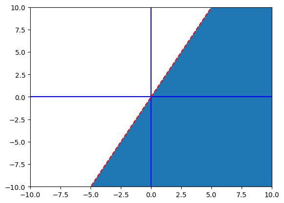
Step 2 - Graphing inequalities - Part 2
The default graph will give you a solid line, but you can change the type of line and the color. As 'b' is for a solid blue line, 'b--' will be a dashed blue line and 'r--' will display a dashed red line. Change the code to graph a dashed red line.
import matplotlib.pyplot as plt
import numpy as np

xmin = -10
xmax = 10
ymin = - 10
ymax = 10
points = 2*(xmax-xmin)
x = np.linspace(xmin,xmax,points)

fig, ax = plt.subplots()
plt.axis([xmin,xmax,ymin,ymax]) # window size
plt.plot([xmin,xmax],[0,0],'b') # blue x axis
plt.plot([0,0],[ymin,ymax], 'b') # blue y axis

y1 = 2*x

# Only change the next line:
plt.plot(x, y1, 'r--')

plt.fill_between(x, y1, ymin)
plt.show()


# Only change code above this line
import math_code_test_c as test
test.step02(In[-1].split('# Only change code above this line')[0])
Code test passed
Go on to the next step
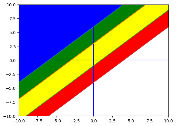
Step 3 - Making Art with Graphs
Now plot four inequalities on the graph, in a pattern. Notice how you only need to define the x values once. In the fill_between() function notice a fourth argument, facecolor=, to indicate a different color for the shaded area. The color name in single quotes, like 'green' or 'yellow' or any common color name. Run the code to see the pattern, then reverse the order of the colors and run it again.
import matplotlib.pyplot as plt
import numpy as np

xmin = -10
xmax = 10
ymin = - 10
ymax = 10
points = 2*(xmax-xmin)
x = np.linspace(xmin,xmax,points)

fig, ax = plt.subplots()
plt.axis([xmin,xmax,ymin,ymax]) # window size
plt.plot([xmin,xmax],[0,0],'b') # blue x axis
plt.plot([0,0],[ymin,ymax], 'b') # blue y axis

# Only change the lines indicated below

# line 1
y1 = x+6
plt.plot(x, y1)
plt.fill_between(x, y1, 10, facecolor='blue') # change this line

# line 2
y2 = x+3
plt.plot(x, y2)
plt.fill_between(x, y2, y1, facecolor='green') # change this line

# line 3
y3 = x-1
plt.plot(x, y3)
plt.fill_between(x, y3, y2, facecolor='yellow') # change this line

# line 4
y4 = x-4
plt.plot(x, y4)
plt.fill_between(x, y4, y3, facecolor='red') # change this line

plt.show()


# Only change code above this line
import math_code_test_c as test
test.step03(In[-1].split('# Only change code above this line')[0])
Code test passed
Go on to the next step
Step 4 - Monomials
A monomial means "one thing" or one term. In a math equation, each term has a sign, a coefficient, and a variable to an exponent. Here are some examples: In the term -3x2 you can see that the sign is negative, the coefficient is 3, the variable is x, the exponent is 2. The term x also has all of these parts: the sign is positive, the coefficient is 1, the variable is x, and the exponent is 1. In the term 5, the sign is positive, the coefficient is 5, the variable is still x, and the exponent is zero (notice that you don't need to write some of these parts, like x0). You can use sympy to display monomials nicely. Just run the code to see how this looks.
from sympy import symbols, Eq

x = symbols('x')
eq1 = Eq(-2*x**3 , -16)
display(eq1)


# Just run this code
import math_code_test_c as test
test.step00()
\displaystyle - 2 x^{3} = -16
Code test passed
Go on to the next step
Step 5 - Polynomials
A "monomial" is one thing. A "binomial" is two things. A "trinomial" is three things. A "polynomial" is many things. In standard form, x is the variable; you put your terms in order from highest exponent to lowest; refer to the coefficients with letters in alphabetical order; and set all of this equal to y (because it is a function that you can graph). Example: y = ax4 + bx3 + cx2 + dx + e
Write code to prompt for integer input and display a polynomial. Remember to use the ** for exponents. Parts of this are already done for you.
from IPython.display import display, Math
from sympy import *

x,y = symbols('x y')

a = int(input("Enter coefficient A: "))
b = int(input("Enter coefficient B: "))
# continue this to prompt for variables c and d
c = int(input("Enter coefficient C: "))
d = int(input("Enter coefficient D: "))

# change the next line to display the full polynomial
y = a*x**3 + b*x**2 + c*x + d

print("Here is your equation:")
display(Math("y = " + latex(y)))


# Only change code above this line
import math_code_test_c as test
test.step05(In[-1].split('# Only change code above this line')[0])
Enter coefficient A:  3
Enter coefficient B:  56
Enter coefficient C:  2
Enter coefficient D:  6


Here is your equation:
\displaystyle y = 3 x^{3} + 56 x^{2} + 2 x + 6
Code test passed
Go on to the next step
Step 6 - Interactive Polynomial Graph
For this polynomial, y = ax2 + bx + c, you can move the sliders to adjust the coefficients and see how that affects the graph. Notice how the f() function takes two arguments and the interactive() function defines two sliders. Run this code and interact with it. Then add the third coefficient ("c") by changing three things: the def line so that the function takes three arguments, the plt.plot line so that it includes "+ c", and the interactive line to include a third slider.
%matplotlib inline
from ipywidgets import interactive
import matplotlib.pyplot as plt
import numpy as np

# Change the next line:
def f(a, b, c):
    plt.axis([-10,10,-10,10]) # window size
    plt.plot([-10,10],[0,0],'k') # blue x axis
    plt.plot([0,0],[-10,10], 'k') # blue y axis
    x = np.linspace(-10, 10, 200)
    plt.plot(x, a*x**2+b*x+c) # Change this line
    plt.show()

# Change the next line:
interactive_plot = interactive(f, a=(-9, 9), b=(-9, 9), c=(-9, 9))
display(interactive_plot)


# Only change code above this line
import math_code_test_c as test
test.step06(In[-1].split('# Only change code above this line')[0])
interactive(children=(IntSlider(value=0, description='a', max=9, min=-9), IntSlider(value=0, description='b', …


Code test passed
Go on to the next step
Step 7 - Exponential Functions
The general formula for an exponential function is y = a*b^{x} (where a and b are constants and x is the variable in the exponent). The shape of exponential graphs, especially when not drawn to scale, are very consistent, so the numerical values are more important to calculate. Things that grow exponentially include populations, investments, and other "percent increase" situations. Run this code and use the sliders to see the slight changes. Notice the scale. Then change the slider so that a has negative values from -9 to -1 and see how that changes the graph.
%matplotlib inline
from ipywidgets import interactive
import matplotlib.pyplot as plt
import numpy as np

xmin = -10
xmax = 10
ymin = -100
ymax = 100

def f(a, b):
    plt.axis([xmin,xmax,ymin,ymax]) # window size
    plt.plot([xmin,xmax],[0,0],'k') # x axis
    plt.plot([0,0],[ymin,ymax], 'k') # y axis
    x = np.linspace(xmin, xmax, 1000)
    plt.plot(x, a*b**x)
    plt.show()

# Only change the next line:
interactive_plot = interactive(f, a=(-9, -1), b=(1, 9))
display(interactive_plot)


# Only change code above this line
import math_code_test_c as test
test.step07(In[-1].split('# Only change code above this line')[0])
interactive(children=(IntSlider(value=-5, description='a', max=-1, min=-9), IntSlider(value=5, description='b'…


Code test passed
Go on to the next step
Step 8 - Percent Increase
One formula for calculating a percent increase is A = P(1 + r)t where A would be the y value on a graph and t would be the x value. A is the annuity, which is the amount you have at the end. P is the principle, which is the amount you have at the beginning. R (usually not capitalized) is the rate, a percent converted to a decimal. The exponent t represents time, usually in years. The code already prompts for P, r and t, so use those variables to calculate the annuity value.
p = float(input("Starting amount = "))
r = float(input("Enter the percentage rate, converted to a decimal: "))
t = float(input("How many years will this investment grow? "))

# Change the next line to calculate the annuity
a = p*(1+r)**t

print("The annuity is ", a)


# Only change code above this line
import math_code_test_c as test
test.step08(In[-1].split('# Only change code above this line')[0])
Starting amount =  100
Enter the percentage rate, converted to a decimal:  0.06
How many years will this investment grow?  5


The annuity is  133.82255776000002

Code test passed
Go on to the next step
Step 9 - Percent Decrease
The percent decrease formula is very similar, except you subtract the rate, so the formula is A = P(1 - r)t. Some things that decrease by a percent include car values, decay of some elements, and sales discounts. Use the existing variables to calculate the final value (a).
p = float(input("Starting amount = "))
r = float(input("Enter the percentage rate, converted to a decimal: "))
t = float(input("How many years will this decrease continue? "))

# Change the next line to calculate the final amount
a = p*(1-r)**t

print("The final amount is ", a)

# Only change code above this line
import math_code_test_c as test
test.step09(In[-1].split('# Only change code above this line')[0])
Starting amount =  2323
Enter the percentage rate, converted to a decimal:  0.12
How many years will this decrease continue?  27


The final amount is  73.63450265803228

Code test passed
Go on to the next step
Step 10 - Compound Interest
When you use percent increase formulas for money in the bank, it's called compound interest. The amount of money you earn beyond the original principle is the interest. When the bank calculates the interest and adds it to the principle, that process is called compounding and it can happen any number of times per year. The formula is A = P(1 + \frac{r}{n})nt where n is the number of times the bank compounds the money per year. Notice that if n = 1 then this formula is the same as the formula from an earlier step. Write the code to calculate the annuity (hint: use extra parentheses).
p = float(input("Starting amount: "))
r = float(input("Percentage rate, converted to a decimal: "))
t = float(input("Number of years this investment will grow: "))
n = int(input("Number of times compounded per year: "))

# Change the next line to calculate the annuity
annuity = p*(1+(r/n))**(n*t)

print("The annuity is ", annuity)


# Only change code above this line
import math_code_test_c as test
test.step10(In[-1].split('# Only change code above this line')[0])
Starting amount:  100
Percentage rate, converted to a decimal:  0.12
Number of years this investment will grow:  4
Number of times compounded per year:  4


The annuity is  160.47064390987882

Code test passed
Go on to the next step
Step 11 - Continuous Growth
In the first formula, A = P(1 + r)t, money is compounded annually.
In the second formula, A = P(1 + \frac{r}{n})^{nt}, money is compounded n times per year.
As n gets to be a really big number, you get a different formula, A = Pe$^{rt}$, for continuous growth.
In this formula, e is a constant, about equal to 2.718281828. The following code already prompts for the four variables once. Use those variables to compare the annuity from the three formulas. Notice you need to import math to use math.e (the best approximation of e).
import math

p = float(input("Principle: "))
r = float(input("Rate: "))
t = int(input("Time: "))
n = int(input("N: "))

# Only change the following three formulas:
a_annual = p*(1+r)**t
a_n_times = p*(1+r/n)**(n*t)
a_continuous = p*math.e**(r*t) # use math.e in this formula

# Only change the code above this line

print("Compounded annually, anuity = ", a_annual)
print("Compounded ", n, "times per year, anuity = ", a_n_times)
print("Compounded continuously, anuity = ", a_continuous)


# Only change code above this line
import math_code_test_c as test
test.step11(In[-1].split('# Only change code above this line')[0])
Principle:  100
Rate:  0.08
Time:  5
N:  12


Compounded annually, anuity =  146.93280768000005
Compounded  12 times per year, anuity =  148.9845708301605
Compounded continuously, anuity =  149.18246976412703

Code test passed
Go on to the next step
Step 12 - Investments
If you have an investment where you contrubute money every month and the value also increases by a consistent percentage, you can create a loop to calculate the accumulated value. In each iteration, use the simple interest formula: interest = principle * rate * time. (Hint: for one month, t = \frac{1}{12} or you can just divide by 12.)
p = float(input("Starting amount: "))
r = float(input("Annual percentage rate: "))
t = int(input("Number of years: "))
monthly = float(input("Monthly contribution: "))

# Hint: keep updating this annuity variable in the loop
annuity = p

# Each iteration of the loop represents one month
for a in range(12*t):
    annuity = annuity + monthly
    # Change the next line to calculate the interest
    interest = annuity * (r/12)
    annuity = annuity + interest

# Keep this line:
print("Annuity = ", annuity)


# Only change code above this line
import math_code_test_c as test
test.step12(p,r,t,monthly,annuity)
Starting amount:  100
Annual percentage rate:  0.08
Number of years:  5
Monthly contribution:  10


Annuity =  888.6515903655937

Code test passed
Go on to the next step
Step 13 - Mortgage Payments
When borrowing a large amount of money over a long period of time, the formula to calculate monthly payments gets complicated. Here it is:
monthly payment = P$\frac{\frac{r}{12}(1 + \frac{r}{12})^{12t}}{(1 + \frac{r}{12})^{12t} - 1}$ where, as usual, P is the principle, r is the annual interest rate (as a decimal), and t is the time in years. Write the code to prompt for these variables and calculate the monthly payment. Hint: Use other variables and do this in steps.
p = float(input("Amount borrowed: "))
r = float(input("Annual percentage rate: "))
t = float(input("Number of years: "))

# Write your code here and change the pmt variable
common = (1 + (r/12))**(12*t)
pmt = p*((r/12)*common)/(common-1)


print("Monthly payment = $", pmt)


# Only change code above this line
import math_code_test_c as test
test.step13(p,r,t,pmt)
Amount borrowed:  1000
Annual percentage rate:  0.12
Number of years:  5


Monthly payment = $ 22.24444768490176

Code test passed
Go on to the next step
Step 14 - Exponents and Logarithms
Exponential functions and logarithmic functions are inverses of each other. Here is an example: 24 = 16 and log216 = 4. Both have the same information rearranged in different ways. If you had 24 = x you would be able to do that easily, but if you had 2x = 16 it would be more difficult. You could write that last equation as a logarithm: log216 = x. In Python, you would write this as math.log(16,2). In both cases, you would read it as "the log, base 2, of 16" and the answer would be an exponent. The logarithm is especially useful when the exponent is not a nice integer. Write code to prompt for the base and the result, then use logarithms to calculate the exponent.
import math

base = float(input("base: "))
result = float(input("result: "))

# Just change the next line:
exp = math.log(result, base)

print("exponent = ", exp)


# Only change code above this line
import math_code_test_c as test
test.step14(In[-1].split('# Only change code above this line')[0])
base:  2
result:  24


exponent =  4.584962500721157

Code test passed
Go on to the next step
Step 15 - Natural Logs
If you know the rate, how long will it take for something to double?
Start with the continuous growth formula:
A = Pert
If annuity is two times the principle, divide both sides by P
and get this:
2 = ert
Because of the base e, take the natural log of both sides and get this:
ln(2) = rt
Then divide by r to solve for t or divide by t to solve for r. In Python, use math.log() with one argument and no base to calculate natural log (which is a logarithm with base e). So the natural log of 2 is math.log(2). Just run the code to see this example.
import math

r = float(input("Enter the annual rate as a decimal: \n"))
t = math.log(2)/r
print("Your money will double in ", t, " years")


# Just run this code
import math_code_test_c as test
test.step00()
Enter the annual rate as a decimal:
 0.05


Your money will double in  13.862943611198904  years
Code test passed
Go on to the next step
Step 16 - Common Logs
The common log is base 10, because that is our number system. Run this code a few times to see how the exponents relate to moving the decimal point to get the resulting number. Notice the floor function. Then take out the floor function to see the exact logarithm.
import math

n = input('Enter a number with several digits or several decimal places: ')
n = float(n)


# Run the code then change the next line:
exp = math.log(n, 10)

# This avoids a weird Python quirk:
if n==1000:
    exp = 3;

print("exponent = ", exp)


# Only change code above this line
import math_code_test_c as test
test.step16(In[-1].split('# Only change code above this line')[0])
Enter a number with several digits or several decimal places:  1232.43524


exponent =  3.090764107949619

Code test passed
Go on to the next step
Step 17 - Scientific Notation
Scientific Notation is a way of writing very large or very small numbers without all of the zeros or decimal places. For example, 45,000,000 could be written as 4.5 x 10⁷ in scientific notation and 0.00000045 could be written as 4.5 x 10⁻⁷. The notation requires base 10, so it will always use the structure n * 10x where n is one digit then the decimal point. Change the code below to print each number in scientific notation. Determine the value of each variable by counting (not writing code). You will automate this process in the next step.
a = 156000000000
b = 0.000000000413

# Change the code below this line

a1 = 1.56
a2 = 11
b1 = 4.13
b2 = -10

print(a, " = ", a1, "* 10^", a2)

print(b, " = ", b1, "* 10^", b2)


# Only change code above this line
import math_code_test_c as test
test.step17(b1,b2)
156000000000  =  1.56 * 10^ 11
4.13e-10  =  4.13 * 10^ -10

Code test passed
Go on to the next step
Step 18 - Logs and Scientific Notation
Writing code for scientific notation, you will make use of logarithms with base 10. Remember that scientific notation is in the form n * 10x where n is one digit and then a decimal. To convert a number to scientific notation, take the log of the number and use the floor() function to get the expoenent (just as you did in a previous step). Divide the original number by 10 to that exponent and you get n (hint: dividing by 10x is the same as multiplying by 10-x). Rounding is usually necessary. Write the code to convert numbers to scientific notation.
import math

a = .00000000000234
b = 12300000000000

# Use these three lines as a model
x1 = math.floor(math.log(a,10))
n1 = round(a*10**(-x1),2)
print("a = ", n1, "* 10^", x1)

# Change the next two lines to match the model
x2 = math.floor(math.log(b, 10))
n2 = round(b*10**(-x2), 2)
print("b = ", n2, "* 10^", x2)


# Only change code above this line
import math_code_test_c as test
test.step18(In[-1].split('# Only change code above this line')[0])
a =  2.34 * 10^ -12
b =  1.23 * 10^ 13

Code test passed
Go on to the next step
Step 19 - Scientific Notation Conversion
Now ask for a number as input, and write the code to convert that number into scientific notation. You can re-use code you used in the previous step, using n and x as variables to print n * 10^x.
import math

a = float(input('Enter a number to convert to scientific notation: '))

# write your code here
n = math.floor(math.log(a, 10))
x = round(a/10**n, 2)
print(f"a = {x}*10^{n}")

# Only change code above this line
import math_code_test_c as test
test.step19(In[-1].split('# Only change code above this line')[0])
Enter a number to convert to scientific notation:  0.005


a = 5.0*10^-3

You should use x = math.floor(math.log(a,10)) in your code
You should use n = round(a*10**(-x),2) in your code
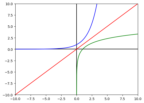
Step 20 - Graphing Exponents and Logs
When not writing code, the natural log is written as "ln" and it means a logarithm with base e. Like any pair of inverse functions, the line y = ex and the line y = ln(x) are mirrored over the line y = x. Because of the np.linspace() function in this code, np.log() works, but math.log() does not work here. Both log() functions in Python use e as the base by default. When using the numpy library, use np.log10() for base 10, np.log2() for base 2, etc. Because log functions can only have positive x values, the np.linspace() function will define a positive range for the log() function. Run this code, then change the blue line function to graph y = 2x and change the green line function to graph y = log2x and notice the similarities between the graphs.
import matplotlib.pyplot as plt
import numpy as np
import math

xmin = -10
xmax = 10
ymin = -10
ymax = 10
plt.axis([xmin,xmax,ymin,ymax]) # window size
plt.plot([xmin,xmax],[0,0],'k') # x axis
plt.plot([0,0],[ymin,ymax], 'k') # y axis

# Same x values for two lines
x1 = np.linspace(xmin, xmax, 1000)

# Blue line for y = e^x
plt.plot(x1, 2**x1, 'b')  # Change this line

# Red line for y = x
plt.plot(x1, x1, 'r')

# Different x values for y = log(x) because x > 0
x2 = np.linspace(.001, xmax, 500)

# Green line for y = log(x)
plt.plot(x2, np.log2(x2), 'g')  # Change this line

plt.show()


# Only change code above this line
import math_code_test_c as test
test.step20(In[-1].split('# Only change code above this line')[0])
Code test passed
Go on to the next step
Step 21 - Log Application - pH Scale
The pH scale, for measuring acids and bases, is a logarithmic scale. The negative log of the hydrogen concentration is the pH. Example: if the hydrogen concentration is .007 then that would be 7 * 10-3 and therefore a pH of 3. Write the code to prompt for hydrogen concentration and then print the pH. Hint: the ceiling function (math.ceil()) works better than rounding here.
import math

decimal = float(input("Enter the hydrogen concentration as a decimal number: "))

# Write your code here
h = math.ceil(-math.log(decimal, 10))

print("pH = ", h)

# Only change code above this line
import math_code_test_c as test
test.step21(In[-1].split('# Only change code above this line')[0])
Enter the hydrogen concentration as a decimal number:  0.007


pH =  3

Code test passed
Step 22 - Functions for the Project
Define a function for calculating mortgage payments and a function for calculating investment balance. Use code you wrote in earlier steps. Each function should prompt for input and print the output.
# Write your code here
def monthly_mortage_payment():
    print("Provide following information to calculate monthly mortgage payment:")
    p = float(input("Loan amount: "))
    r = float(input("Rate of inerest (in decimal): "))
    t = float(input("Loan duration (in years): "))
    common = (1+ (r/12))**(t*12)
    monthly_payment = p * (((r/12)*common)/(common-1))
    print("Monthly payment will be:", monthly_payment)

def retirement_corpus():
    print("Provide following information to estimate your retirement savings:")
    s = float(input("Current savings: "))
    r = float(input("Estimated rate of return on investments (in decimal): "))/12
    m = float(input("Monthly savings: "))
    t = float(input("Number of years till retirement: "))

    for i in range(int(t*12)):
        s += m
        s = s + (s*r)

    print("Estimated retirement savings: ", s)
# This step does not have a test
Provide following information to estimate your retirement savings:


Current savings:  0
Estimated rate of return on investments (in decimal):  0.05
Monthly savings:  1300
Number of years till retirement:  40


Estimated retirement savings:  1992092.1458609407
Step 23 - More Functions
Create a function that produces an interactive polynomial graph (with sliders). Use code from an earlier step.
# Write your code here

def f(a, b, c):
    xlo = -100
    xhi = 100
    ylo = -100
    yhi = 100

    plt.clf()
    fig = plt.subplot()
    plt.axis([xlo, xhi, ylo, yhi])
    plt.plot([xlo, xhi], [0, 0], "black")
    plt.plot([0, 0], [ylo, yhi], "black")

    x = np.linspace(xlo, xhi, (xhi-xlo)*5)
    y = a*x**2 + b*x + c
    plt.plot(x, y)

    plt.grid()
    plt.show()

interactive_graph = interactive(f, a=(-10, 10, 0.1), b=(-10, 10, 0.1), c=(-10, 10, 0.1))
interactive_graph
# This step does not have a test
interactive(children=(FloatSlider(value=0.0, description='a', max=10.0, min=-10.0), FloatSlider(value=0.0, des…
Step 24 - New Function
Create a function to print the time required for money to double, given the rate. Use the continuous growth formula from an earlier step.
# Write your code here
def time_to_double():
    r = float(input("Give rate of interest/return (in decimal) to find time to double: "))
    t = round(math.log(2)/r, 2)
    print(f"It will take {t} years for amount to double.")
# This step does not have a test
Give rate of interest/return (in decimal) to find time to double:  0.05


It will take 13.86 years for amount to double.
Step 25 - Certification Project 3
Build a financial app that calculates all of the following:
- Mortgage payment - given principle, rate, time
- Retirement account balance at time of retirement
- Time required for money to double - given the rate
- Rate of growth - given starting value, time, and ending value
# Write your code here
def time_to_double():
    print("Provide following information to determine needed rate of grwoth for given amount to reach desired amount in given time (years): ")
    p = float(input("Current amount: "))
    a = float(input("Desired future amount: "))
    t = float(input("Number of years: "))
    r = round(math.log(a/p)/t, 2)
    print(f"{r*100}% rate of growth is needed for {p} to reach {a} in {t} years.")

rate_of_grwoth()
Provide following information to determine needed rate of grwoth for given amount to reach desired amount in given time (years):


Current amount:  100
Desired future amount:  200
Number of years:  13.8


5.0% rate of growth is needed for 100.0 to reach 200.0 in 13.8 years.
options = [
    (monthly_mortage_payment, "Mortgage payment - given principle, rate, time"),
    (retirement_corpus, "Retirement account balance at time of retirement"),
    (rate_of_grwoth, "Rate of growth - given starting value, time, and ending value"),
    (time_to_double, "Time required for money to double - given the raten")
]

print("What would you like to do?")
[print(o[1]) for o in options]
selected = int(input())

if selected >= 1 and selected <= len(options):
    options[selected-1][0]()
What would you like to do?
Mortgage payment - given principle, rate, time
Retirement account balance at time of retirement
Rate of growth - given starting value, time, and ending value
Time required for money to double - given the raten


 1


Provide following information to calculate monthly mortgage payment:


Loan amount:  1000000
Rate of inerest (in decimal):  0.06
Loan duration (in years):  30


Monthly payment will be: 5995.505251527569