You cannot select more than 25 topics Topics must start with a letter or number, can include dashes ('-') and can be up to 35 characters long.

34 KiB

Raw Permalink Blame History Unescape Escape

Learn Foundational Math 2 by Building Cartesian Graphs
Each of these steps will lead you toward the Certification Project. Once you complete a step, click to expand the next step.

↓ Do this first ↓

Copy this notebook to your own account by clicking the File button at the top, and then click Save a copy in Drive. You will need to be logged in to Google. The file will be in a folder called "Colab Notebooks" in your Google Drive.

Step 0 - Acquire the testing library

Please run this code to get the library file from FreeCodeCamp. Each step will use this library to test your code. You do not need to edit anything; just run this code cell and wait a few seconds until it tells you to go on to the next step.

# You may need to run this cell at the beginning of each new session

!pip install requests

# This will just take a few seconds

import requests

# Get the library from GitHub
url = 'https://raw.githubusercontent.com/edatfreecodecamp/python-math/main/math-code-test-b.py'
r = requests.get(url)

# Save the library in a local working directory
with open('math_code_test_b.py', 'w') as f:
    f.write(r.text)

# Now you can import the library
import math_code_test_b as test

# This will tell you if the code works
test.step01()

Requirement already satisfied: requests in /usr/local/lib/python3.8/dist-packages (2.31.0)
Requirement already satisfied: charset-normalizer<4,>=2 in /usr/local/lib/python3.8/dist-packages (from requests) (3.2.0)
Requirement already satisfied: idna<4,>=2.5 in /usr/lib/python3/dist-packages (from requests) (2.8)
Requirement already satisfied: urllib3<3,>=1.21.1 in /usr/lib/python3/dist-packages (from requests) (1.25.8)
Requirement already satisfied: certifi>=2017.4.17 in /usr/lib/python3/dist-packages (from requests) (2019.11.28)
[33mWARNING: Running pip as the 'root' user can result in broken permissions and conflicting behaviour with the system package manager. It is recommended to use a virtual environment instead: https://pip.pypa.io/warnings/venv[0m[33m
[0m
[1m[[0m[34;49mnotice[0m[1;39;49m][0m[39;49m A new release of pip is available: [0m[31;49m23.1.2[0m[39;49m -> [0m[32;49m23.2.1[0m
[1m[[0m[34;49mnotice[0m[1;39;49m][0m[39;49m To update, run: [0m[32;49mpython3 -m pip install --upgrade pip[0m
Code test Passed
Go on to the next step

Step 1 - Cartesian Coordinates

Learn Cartesian coordinates by building a scatterplot game. The Cartesian plane is the classic x-y coordinate grid (invented by Ren$\acute{e}$ DesCartes) where "x" is the horizontal axis and "y" is the vertical axis. Each (x,y) coordinate pair is a point on the graph. The point (0,0) is the "origin." The x value tells how much to move right (positive) or left (negative) from the origin. The y value tells you how much you move up (positive) or down (negative) from the origin. Notice that you are importing matplotlib to create the graph. The following code just displays one quadrant of the Cartesian graph. Just run this code to see how Python displays a graph.

import matplotlib.pyplot as plt

fig, ax = plt.subplots()
plt.show()

# Just run this code to see a blank graph
import math_code_test_b as test
test.step01()

Code test Passed
Go on to the next step

Step 2 - Cartesian Coordinates (Part 2)

Here you will create a standard window but still not highlight each axis. Run this code once, then change the window size to 20 in each direction and run it again.

import matplotlib.pyplot as plt

fig, ax = plt.subplots()

# Only change the numbers in the next line:
plt.axis([-20,20,-20,20])

plt.show()


# Only change code above this line
import math_code_test_b as test
test.step02(In[-1].split('# Only change code above this line')[0])

Code test passed
Go on to the next step

Step 3 - Graph Dimensions

When you look at this code, you can see how Python sets up window dimensions. You will also notice that it is easier and more organized to define the dimensions as variables. Run the code, then change just the xmax value to 20 and run it again to see the difference.

import matplotlib.pyplot as plt

xmin = -10
xmax = 20
ymin = -10
ymax = 10

fig, ax = plt.subplots()
plt.axis([xmin,xmax,ymin,ymax]) # window size
plt.show()

# Only change code above this line
import math_code_test_b as test
test.step03(In[-1].split('# Only change code above this line')[0])

Code test passed
Go on to the next step

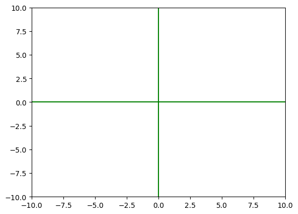
Step 4 - Displaying Axis Lines

Notice the code to plot a line for the x axis and a line for the y axis. The 'b' makes the line blue. Run the code, then change each 'b' to 'g' to make the lines green.

import matplotlib.pyplot as plt

xmin = -10
xmax = 10
ymin = -10
ymax = 10

fig, ax = plt.subplots()
plt.axis([xmin,xmax,ymin,ymax]) # window size
plt.plot([xmin,xmax],[0,0],'g') # blue x axis
plt.plot([0,0],[ymin,ymax], 'g') # blue y axis

plt.show()

# Only change code above this line
import math_code_test_b as test
test.step04(In[-1].split('# Only change code above this line')[0])

Code test passed
Go on to the next step

Step 5 - Plotting a Point

Now you will plot a point on the graph. Notice the 'ro' makes the point a red dot. Run the code, then change the location of the point to (-5,1) and run it again. Keep the window size the same. Notice the difference between plotting a point and plotting a line.

import matplotlib.pyplot as plt

xmin = -10
xmax = 10
ymin = -10
ymax = 10

fig, ax = plt.subplots()
plt.axis([xmin,xmax,ymin,ymax]) # window size
plt.plot([xmin,xmax],[0,0],'b') # blue x axis
plt.plot([0,0],[ymin,ymax], 'b') # blue y axis

# Change only the numbers in the following line:
plt.plot([-5],[1], 'ro')

plt.show()


# Only change code above this line
import math_code_test_b as test
test.step05(In[-1].split('# Only change code above this line')[0])

Code test passed
Go on to the next step

Step 6 - Plotting Several Points

You have actually been using arrays to plot each singular point so far. In this step, you will see an array of x values and an array of y values defined before the plot statement. Notice that these two short arrays create one point: (4,2). Add two numbers to each array so that it also plots points (1,1) and (2,5).

import matplotlib.pyplot as plt

# only change the next two lines:
x = [4, 1, 2]
y = [2, 1, 5]

# Only change code above this line

xmin = -10
xmax = 10
ymin = -10
ymax = 10

fig, ax = plt.subplots()
plt.axis([xmin,xmax,ymin,ymax]) # window size
plt.plot([xmin,xmax],[0,0],'b') # blue x axis
plt.plot([0,0],[ymin,ymax],'b') # blue y axis

plt.plot(x, y, 'ro') # red points
plt.show()


# Only change code above this line
import math_code_test_b as test
test.step06(In[-1].split('# Only change code above this line')[0])

Code test passed
Go on to the next step

Step 7 - Plotting Points and Lines

Notice the subtle difference between plotting points and lines. Each plot() statement takes an array of x values, an array of y values, and a third argument to tell what you are plotting. The default plot is a line. The letters 'r' and 'b' (and 'g' and a few others) indicate common colors. The "o" in 'ro' indicates a dot, where 'rs' would indicate a red square and 'r^' would indicate a red triangle. Plot a red line and two green squares.

import matplotlib.pyplot as plt

# Use these numbers:
linex = [2,4]
liney = [1,5]
pointx = [1,6]
pointy = [6,3]

# Keep these lines:
xmin = -10
xmax = 10
ymin = -10
ymax = 10

fig, ax = plt.subplots()
plt.axis([xmin,xmax,ymin,ymax]) # window size
plt.plot([xmin,xmax],[0,0],'b') # blue x axis
plt.plot([0,0],[ymin,ymax], 'b') # blue y axis

# Change the next two lines:
plt.plot(linex, liney, 'r')
plt.plot(pointx, pointy, 'gs')

plt.show()


# Only change code above this line
import math_code_test_b as test
test.step07(In[-1].split('# Only change code above this line')[0])

Code test passed
Go on to the next step

Step 8 - Making a Scatterplot Game

To make the game, you can make a loop that plots a random point and asks the user to input the (x,y) coordinates. Notice the for loop that runs three rounds of the game. Run the code, play the game, then you can go on to the next step.

import matplotlib.pyplot as plt
import random

score = 0

xmin = -8
xmax = 8
ymin = -8
ymax = 8

fig, ax = plt.subplots()

for i in range(0,3):
    xpoint = random.randint(xmin, xmax)
    ypoint = random.randint(ymin, ymax)
    x = [xpoint]
    y = [ypoint]
    plt.axis([xmin,xmax,ymin,ymax]) # window size
    plt.plot([xmin,xmax],[0,0],'b') # blue x axis
    plt.plot([0,0],[ymin,ymax], 'b') # blue y axis
    plt.plot(x, y, 'ro')
    print(" ")
    plt.grid() # displays grid lines on graph
    plt.show()
    guess = input("Enter the coordinates of the red point point: \n")
    guess_array = guess.split(",")
    xguess = int(guess_array[0])
    yguess = int(guess_array[1])
    if xguess == xpoint and yguess == ypoint:
        score = score + 1

print("Your score: ", score) # notice this is not in the loop


# Only change code above this line
import math_code_test_b as test
test.step08(score)

Enter the coordinates of the red point point: 
 -3, 0

Enter the coordinates of the red point point: 
 -7, 0

Enter the coordinates of the red point point: 
 2, 7


Your score:  3
You scored 3 out of 3. Good job!
You can go on to the next step

Step 9 - Graphing Linear Equations

Besides graphing points, you can graph linear equations (or functions). The graph will be a straight line, and the equation will not have any exponents. For these graphs, you will import numpy and use the linspace() function to define the x values. That function takes three arguments: starting number, ending number, and number of steps. Notice the plot() function only has two arguments: the x values and a function (y = 2x - 3) for the y values. Run this code, then use the same x values to graph y = -x + 3.

import matplotlib.pyplot as plt
import numpy as np

xmin = -10
xmax = 10
ymin = -10
ymax = 10

fig, ax = plt.subplots()
plt.axis([xmin,xmax,ymin,ymax]) # window size
plt.plot([xmin,xmax],[0,0],'b') # blue x axis
plt.plot([0,0],[ymin,ymax], 'b') # blue y axis

x = np.linspace(-9,9,36)

# Only change the next line to graph y = -x + 3
plt.plot(x, -x + 3)



plt.show()


# Only change code above this line
import math_code_test_b as test
test.step09(In[-1].split('# Only change code above this line')[0])

Code test passed
Go on to the next step

Step 10 - Creating Interactive Graphs

Like the previous graphs, you will graph a line. This time, you will create two sliders to change the slope and the y intecept. Notice the additional imports and other changes: You define a function with two arguments. All of the graphing happens within that f(m,b) function. The interactive() function calls your defined function and sets the boundaries for the sliders. Run this code then adjust the sliders and notice how they affect the graph.

%matplotlib inline
from ipywidgets import interactive
import matplotlib.pyplot as plt
import numpy as np

# Define the graphing function
def f(m, b):
    xmin = -10
    xmax = 10
    ymin = -10
    ymax = 10
    plt.axis([xmin,xmax,ymin,ymax]) # window size
    plt.plot([xmin,xmax],[0,0],'black') # black x axis
    plt.plot([0,0],[ymin,ymax], 'black') # black y axis
    plt.title('y = mx + b')
    x = np.linspace(-10, 10, 1000)
    plt.plot(x, m*x+b)
    plt.show()

# Set up the sliders
interactive_plot = interactive(f, m=(-9, 9), b=(-9, 9))
interactive_plot


# Just run this code and use the sliders
import math_code_test_b as test
test.step01()
interactive_plot

Code test Passed
Go on to the next step





interactive(children=(IntSlider(value=0, description='m', max=9, min=-9), IntSlider(value=0, description='b', …

Step 11 - Graphing Systems

When you graph two equations on the same coordinate plane, they are a system of equations. Notice how the points variable defines the number of points and the linspace() function uses that variable. Run this code to see the graph, then change y2 so that it graphs y = -x - 3.

import matplotlib.pyplot as plt
import numpy as np


xmin = -10
xmax = 10
ymin = -10
ymax = 10
points = 2*(xmax-xmin)

# Define the x values once
x = np.linspace(xmin,xmax,points)

fig, ax = plt.subplots()
plt.axis([xmin,xmax,ymin,ymax]) # window size
plt.plot([xmin,xmax],[0,0],'b') # blue x axis
plt.plot([0,0],[ymin,ymax], 'b') # blue y axis

# line 1
y1 = 2*x
plt.plot(x, y1)

# line 2
y2 = -x - 3
plt.plot(x, y2)

plt.show()


# Only change code above this line
import math_code_test_b as test
test.step11(In[-1].split('# Only change code above this line')[0])

Code test passed
Go on to the next step

Step 12 - Systems of Equations - Algebra

In a system of equations, the solution is the point where the two equations intersect, the (x,y) values that work in each equation. To work with algabraic expressions, you will import sympy and define x and y as symbols. If you have two equations and two variables, set each equation equal to zero. The linsolve() function takes the non-zero side of each equation and the variables used. Notice the syntax. Run the code, then change the two equations to solve 2x + y - 15 = 0 and 3x - y = 0.

from sympy import *
x,y = symbols('x y')


# Change the equations in the following line:
print(linsolve([2*x + y - 15, 3*x - y], (x, y)))


# Only change code above this line
import math_code_test_b as test
test.step12(In[-1].split('# Only change code above this line')[0])

{(3, 9)}
 
Code test passed
Go on to the next step

Step 13 - Solutions as Coordinates

The linsolve() function returns a finite set, and you can convert that "finite set" into (x,y) coordinates. Notice how the code parses the solution variable into two separate variables. Just run the code to see how this works.

from sympy import *
x,y = symbols('x y')

# Use variables for each equation
first = x + y
second = x - y

# parse finite set answer as coordinate pair
solution = linsolve([first, second], (x, y))
x_solution = solution.args[0][0]
y_solution = solution.args[0][1]

print("x = ", x_solution)
print("y = ", y_solution)
print(" ")
print("Solution: (",x_solution,",",y_solution,")")


# Just run this code
import math_code_test_b as test
test.step01()

x =  0
y =  0
 
Solution: ( 0 , 0 )
Code test Passed
Go on to the next step

Step 14 - Systems from User Input

For more flexibility, you can get each equation as user input (instead of defining them in the code). Run this code and try it out - to solve any system of two equations.

from sympy import *

x,y = symbols('x y')
print("Remember to use Python syntax with x and y as variables")
print("Notice how each equation is already set equal to zero")
first = input("Enter the first equation: 0 = ")
second = input("Enter the second equation: 0 = ")
solution = linsolve([first, second], (x, y))
x_solution = solution.args[0][0]
y_solution = solution.args[0][1]

print("x = ", x_solution)
print("y = ", y_solution)


# Just run this code and test it with different equations
import math_code_test_b as test
test.step14()

Remember to use Python syntax with x and y as variables
Notice how each equation is already set equal to zero


Enter the first equation: 0 =  1.5*x-6
Enter the second equation: 0 =  -2*x +3*y +9


x =  4.00000000000000
y =  -0.333333333333333
 
If you didn't get a syntax error, code test passed

Step 15 - Solve and graph a system

Now you can put it all together: solve a system of equations, graph the system, and plot a point where the two lines intersect. Notice how this code is not like the previous solving equations code or the graphing code or the user input code. Python uses sympy to get the (x,y) solution and numpy to get the values to graph, so the user inputs nummerical values and the code uses them in two different ways. Think about how you would do this if the user input values for ax + by = c.

from sympy import *
import matplotlib.pyplot as plt
import numpy as np

print("First equation: y = mx + b")
mb_1 = input("Enter m and b, separated by a comma: ")
mb_in1 = mb_1.split(",")
m1 = float(mb_in1[0])
b1 = float(mb_in1[1])

print("Second equation: y = mx + b")
mb_2 = input("Enter m and b, separated by a comma: ")
mb_in2 = mb_2.split(",")
m2 = float(mb_in2[0])
b2 = float(mb_in2[1])

# Solve the system of equations
x,y = symbols('x y')
first = m1*x + b1 - y
second = m2*x + b2 - y
solution = linsolve([first, second], (x, y))
x_solution = round(float(solution.args[0][0]),3)
y_solution = round(float(solution.args[0][1]),3)

# Make sure the window includes the solution
xmin = int(x_solution) - 20
xmax = int(x_solution) + 20
ymin = int(y_solution) - 20
ymax = int(y_solution) + 20
points = 2*(xmax-xmin)

# Define the x values once for the graph
graph_x = np.linspace(xmin,xmax,points)

# Define the y values for the graph
y1 = m1*graph_x + b1
y2 = m2*graph_x + b2

fig, ax = plt.subplots()
plt.axis([xmin,xmax,ymin,ymax]) # window size
plt.plot([xmin,xmax],[0,0],'b') # blue x axis
plt.plot([0,0],[ymin,ymax], 'b') # blue y axis

# line 1
plt.plot(graph_x, y1)

# line 2
plt.plot(graph_x, y2)

# point
plt.plot([x_solution],[y_solution],'ro')

plt.show()
print(" ")
print("Solution: (", x_solution, ",", y_solution, ")")


# Run this code and test it with different equations

First equation: y = mx + b


Enter m and b, separated by a comma:  3, -4


Second equation: y = mx + b


Enter m and b, separated by a comma:  -2, 7

Solution: ( 2.2 , 2.6 )

Step 16 - Quadratic Functions

Any function that involves x² is a "quadratic" function because "x squared" could be the area of a square. The graph is a parabola. The formula is y = ax² + bx + c, where b and c can be zero but a has to be a number. Here is a graph of the simplest parabola.

import matplotlib.pyplot as plt
import numpy as np

xmin = -10
xmax = 10
ymin = -10
ymax = 10
points = 2*(xmax-xmin)
x = np.linspace(xmin,xmax,points)

fig, ax = plt.subplots()
plt.axis([xmin,xmax,ymin,ymax]) # window size
plt.plot([xmin,xmax],[0,0],'b') # blue x axis
plt.plot([0,0],[ymin,ymax], 'b') # blue y axis

y = x**2

plt.plot(x,y)
plt.show()

# Just run this code. The next step will transform the graph
import math_code_test_b as test
test.step01()

Code test Passed
Go on to the next step

Step 17 - Quadratic Function ABC's

Using the parabola formula y = ax² + bx + c, you will change the values of a, b, and c to see how they affect the graph. Run the code and use the sliders to change the values of a and b. Then change the code in the three places indicated to add a slider for c. You may remember this type of interactive graph from an earlier step. Move each slider to see how it affects the graph.

%matplotlib inline
from ipywidgets import interactive
import matplotlib.pyplot as plt
import numpy as np

# Change the next line to include c:
def f(a,b, c):
    plt.axis([-10,10,-10,10]) # window size
    plt.plot([-10,10],[0,0],'k') # blue x axis
    plt.plot([0,0],[-10,10], 'k') # blue y axis
    x = np.linspace(-10, 10, 1000)

    # Change the next line to add c to the end of the function:
    plt.plot(x, a*x**2 + b*x + c)
    plt.show()

# Change the next line to add a slider to change the c value
interactive_plot = interactive(f, a=(-9, 9), b=(-9,9), c=(-9, 9))
interactive_plot


# Run the code once, then change the code and run it again

# Only change code above this line
import math_code_test_b as test
test.step17(In[-1].split('# Only change code above this line')[0])
interactive_plot

Code test passed
Go on to the next step
 





interactive(children=(IntSlider(value=0, description='a', max=9, min=-9), IntSlider(value=0, description='b', …

Step 18 - Quadratic Functions - Vertex

The vertex is the point where the parabola turns around. The x value of the vertex is \frac{-b}{2a} (and then you would calculate the y value to get the point). Write the code to find the vertex, given a, b, and c as inputs. Remember the parabola forumula is y = ax² + bx + c

import matplotlib.pyplot as plt
import numpy as np

# \u00b2 prints 2 as an exponent
print("y = ax\u00b2 + bx + c")

a = float(input("a = "))
b = float(input("b = "))
c = float(input("c = "))

# Write your code here, changing vx and vy
vx = -b/(2*a)
vy = a*vx**2 + b*vx + c


# Only change the code above this line

print(" (", vx, " , ", vy, ")")
print(" ")

xmin = int(vx)-10
xmax = int(vx)+10
ymin = int(vy)-10
ymax = int(vy)+10
points = 2*(xmax-xmin)
x = np.linspace(xmin,xmax,points)

fig, ax = plt.subplots()
plt.axis([xmin,xmax,ymin,ymax]) # window size
plt.plot([xmin,xmax],[0,0],'b') # blue x axis
plt.plot([0,0],[ymin,ymax], 'b') # blue y axis

plt.plot([vx],[vy],'ro') # vertex

x = np.linspace(vx-10,vx+10,100)
y = a*x**2 + b*x + c
plt.plot(x,y)

plt.show()


# Only change code above this line
import math_code_test_b as test
test.step18(In[-1].split('# Only change code above this line')[0])

y = ax² + bx + c


a =  2
b =  1.89
c =  4.28


 ( -0.4725  ,  3.8334875000000004 )

Code test passed
Go on to the next step

Step 19 - Projectile Motion

The path of every projectile is a parabola. For something thrown or launched upward, the a value is -4.9 (meters per second squared); the b value is the initial velocity (in meters per second); the c value is the initial height (in meters); the x value is time (in seconds); and the y value is the height at that time. In this code, change vx and vy to represent the vertex. Plotting that (x,y) vertex point is already in the code.

import matplotlib.pyplot as plt
import numpy as np

a = -4.9
b = float(input("Initial velocity = "))
c = float(input("Initial height = "))

# Change vx and vy to represent the vertex
vx = -b/(2*a)
vy = a*vx**2 + b*vx + c


# Also change the following dimensions to display the vertex
xmin = -10
xmax = 10
ymin = -10
ymax = 10

# You do not need to change anything below this line
points = 2*(xmax-xmin)
x = np.linspace(xmin,xmax,points)
y = a*x**2 + b*x + c

fig, ax = plt.subplots()
plt.axis([xmin,xmax,ymin,ymax]) # window size
plt.plot([xmin,xmax],[0,0],'b') # blue x axis
plt.plot([0,0],[ymin,ymax], 'b') # blue y axis

plt.plot(x,y) # plot the line for the equation
plt.plot([vx],[vy],'ro') # plot the vertex point

print(" (", vx, ",", vy, ")")
print(" ")
plt.show()


# Only change code above this line
import math_code_test_b as test
test.step19(In[-1].split('# Only change code above this line')[0])

Initial velocity =  10
Initial height =  3


 ( 1.0204081632653061 , 8.102040816326529 )

Code test passed
Go on to the next step

Step 20 - Quadratic Functions - C

Like many other functions, the c value (also called the "constant" because it is not a variable) affects the vertical shift of the graph. Run the following code to see how changing the c value changes the graph.

import matplotlib.pyplot as plt
import numpy as np
import time
from IPython import display

x = np.linspace(-4,4,16)
fig, ax = plt.subplots()
cvalue = "c = "

for c in range(10):
    y = -x**2+c
    plt.plot(x,y)
    cvalue = "c = ", c
    ax.set_title(cvalue)
    display.display(plt.gcf())
    time.sleep(0.5)
    display.clear_output(wait=True)

# Just run this code
import math_code_test_b as test
test.step01()

Code test Passed
Go on to the next step

Step 21 - The Quadratic Formula

For a projectile, you also need to find the point when it hits the ground. On a graph, you would call these points the "roots" or "x intercepts" or "zeros" (because y = 0 at these points). The quadratic formula gives you the x value when y = 0. Given a,b and c, here is the quadratic formula:
x = \frac{-b \pm \sqrt{b^2 - 4ac}}{2a} Notice it's the vertex plus or minus something: \frac{-b}{2a} + \frac{\sqrt{b^2 - 4ac}}{2a} and \frac{-b}{2a} - \frac{\sqrt{b^2 - 4ac}}{2a}
Write the code to output two x values, given a, b, and c as input. Use math.sqrt() for the square root.

import math

# \u00b2 prints 2 as an exponent
print("0 = ax\u00b2 + bx + c")
a = float(input("a = "))
b = float(input("b = "))
c = float(input("c = "))
x1 = 0
x2 = 0

# Check for non-real answers:
if b**2-4*a*c < 0:
    print("No real roots")
else:
    # Write your code here, changing x1 and x2
    x1 = (-b + math.sqrt(b**2 - 4*a*c))/(2*a)
    x2 = (-b - math.sqrt(b**2 - 4*a*c))/(2*a)
    print("The roots are ", x1, " and ", x2)



# Only change code above this line
import math_code_test_b as test
test.step21(In[-1].split('# Only change code above this line')[0])

0 = ax² + bx + c


a =  -2
b =  26
c =  20


The roots are  -0.7284161474004804  and  13.72841614740048
 
Code test passed
Go on to the next step

Step 22 - Table of Values

In addition to graphing a function, you may need a table of values. This code shows how to make a simple table of (x,y) values. Run the code, then change the title to "y = 3x + 2" and change the function in the table.

import numpy as np
import matplotlib.pyplot as plt

ax = plt.subplot()
ax.set_axis_off()
title = "y = 3x + 2" # Change this title
cols = ('x', 'y')
rows = [[0,0]]
for a in range(1,10):
    rows.append([a, 3*a+2]) # Change only the function in this line

ax.set_title(title)
plt.table(cellText=rows, colLabels=cols, cellLoc='center', loc='upper left')
plt.show()


# Only change code above this line
import math_code_test_b as test
test.step22(In[-1].split('# Only change code above this line')[0])

Code test passed
Go on to the next step

Step 23 - Projectile Game

Learn quadratic functions by building a projectile game. Starting at (0,0) you launch a toy rocket that must clear a wall. You can randomize the height and location of the wall. The goal is to determine what initial velocity would get the rocket over the wall. Bonus: make an animation of the path of the rocket.

# Write your code here
fix = plt.subplot()
xlo = -2
xhi = 20
ylo = -20
yhi = 120
plt.axis([xlo, xhi, ylo, yhi])
plt.plot([0, 0], [ylo, yhi], "black")
plt.plot([xlo, xhi], [0, 0], "black")
wall_distance = random.randint(2, xhi-2)
wall_height = random.randint(2, yhi-20)
plt.plot([wall_distance, wall_distance], [0, wall_height], "brown")
plt.grid()
display.display(plt.gcf())

x = np.linspace(0, xhi, xhi*1000)
# a = -4.9
a = -2
c = 0
# b = float(input("We are standing at origin (0, 0), guess velocity at which we need to throw ball to cross the wall: "))
b = 1
while a*wall_distance**2 + b*wall_distance + c < wall_height:
    b += 1
plt.title(f"Velocity of {b} should suffice when wall of {wall_height} height is {wall_distance} distance away.")
y = a*x**2 + b*x + c
x2 = []
y2 = []
for i in range(len(y)):
    if y[i] < 0:
        break
    x2.append(x[i])
    y2.append(y[i])

time.sleep(0.5)
display.clear_output(wait=True)
plt.plot(x2, y2, "b")

ball = plt.plot([x2[0]], [y2[0]], 'ro')[0]

for i in range(1, len(x2)):
    if i%1000 != 0 and i < len(x2) - 2:
        continue
    display.display(plt.gcf())
    time.sleep(0.5)
    display.clear_output(wait=True)
    ball.remove()
    ball = plt.plot([x2[i]], [y2[i]], 'ro')[0]

display.display(plt.gcf())
time.sleep(0.5)
display.clear_output(wait=True)
# This step does not have a test

Step 24 - Define Graphing Functions

Building on what you have already done, create a menu with the following options:

Display the graph and a table of values for any "y=" equation input
Solve a system of two equations without graphing
Graph two equations and plot the point of intersection
Given a, b and c in a quadratic equation, plot the roots and vertex

Then think about how you will define a function for each item.

# Write your code here
from sympy.parsing.sympy_parser import parse_expr
def table_and_graph():
    x, y = symbols("x y")
    eq = input("y = ")
    expr = parse_expr(eq)
    xlo = -10
    xhi = 10
    density = 5
    points = (xhi-xlo) * density
    x_inputs = np.linspace(xlo, xhi, points)
    y_outputs = []
    for n in x_inputs:
        y_outputs.append(expr.evalf(subs={x: n}))
    
    ax = plt.subplot()
    ax.set_axis_off()
    title = f"y = {eq}"
    cols = ('x', 'y')
    rows = []
    for i in range(xlo, xhi + 1):
        rows.append([f"{i:.2f}", f"{round(float(expr.evalf(subs={x: i})), 2):.2f}"])
    
    ax.set_title(title)
    plt.table(cellText=rows, colLabels=cols, cellLoc='center', loc='upper left')
    plt.show()
    
    fig, axis = plt.subplots()
    fig_min = float(min(min(x_inputs), min(y_outputs)))
    fig_max = float(max(max(x_inputs), max(y_outputs)))
    plt.axis([fig_min, fig_max, fig_min, fig_max])
    plt.plot([fig_min, fig_max], [0, 0], "black")
    plt.plot([0, 0], [fig_min, fig_max], "black")
    plt.plot(x_inputs, y_outputs, "b")
    plt.show()

def solve_system_of_equations():
    x, y = symbols("x y")
    eq1 = input("First euqation: 0 = ")
    eq2 = input("Second equation: 0 = ")
    solutions = solve([eq1, eq2], [x, y])
    if len(solutions):
        print("Euqations intercept at:")
        for solution in solutions:
            # WARNING: this will raise error for complex numbers
            print(f"({float(solution[0])}, {float(solution[1])})")
    else:
        print("Give equations do not intercept")

def equations_intercept():
    x, y = symbols("x y")
    eq1 = input("First euqation: 0 = ")
    eq2 = input("Second equation: 0 = ")
    solutions = solve([eq1, eq2], [x, y])
    if len(solutions) == 0:
        print("Equations do not intercept")
        return
    x_intercept_1 = float(solutions[0][0])
    y_intercept_1 = float(solutions[0][1])
    xlo = x_intercept_1 - 20
    xhi = x_intercept_1 + 20
    ylo = y_intercept_1 - 20
    yhi = y_intercept_1 + 20
    density = 5
    x_inputs = [i for i in np.arange(xlo, xhi+0.2, 0.2)]
    y_solver1 = solve(eq1, y)[0]
    y_solver2 = solve(eq2, y)[0]
    y_ouputs_1 = [float(y_solver1.evalf(subs={x: i})) for i in x_inputs]
    y_ouputs_2 = [float(y_solver2.evalf(subs={x: i})) for i in x_inputs]
    fig, axis = plt.subplots()
    plt.axis([xlo, xhi, ylo, yhi])
    plt.plot([xlo, xhi], [0, 0], "black")
    plt.plot([0, 0], [ylo, yhi], "black")
    plt.plot(x_inputs, y_ouputs_1, "blue")
    plt.plot(x_inputs, y_ouputs_2, "orange")
    for solution in solutions:
        plt.plot([solution[0]], [solution[1]], "ro")
    plt.show()

def quadratic_eq_roots_and_vertex():
    a = float(input("a = "))
    b = float(input("b = "))
    c = float(input("c = "))
    vertex_x = -b/(2*a)
    vertex_y = a*vertex_x**2 + b*vertex_x + c
    root_1 = 0
    root_2 = 0
    has_roots = b**2 - 4*a*c >= 0
    if has_roots:
        root_1 = vertex_x + (math.sqrt(b**2 - 4*a*c)/(2*a))
        root_2 = vertex_x - (math.sqrt(b**2 - 4*a*c)/(2*a))
    else:
        print("Given quadratic equation has no roots i.e. do not intercept x-axis at all")
    
    xlo = root_1 - 20 if has_roots else vertex_x - 20
    xhi = root_2 + 20 if has_roots else vertex_x + 20
    ylo = -20 - abs(root_2-root_1) if has_roots else vertex_y - 20
    yhi = 20 + abs(root_2-root_1) if has_roots else vertex_y + 20
    fig, axis = plt.subplots()
    plt.axis([xlo, xhi, ylo, yhi])
    plt.plot([xlo, xhi], [0, 0], "black")
    plt.plot([0, 0], [ylo, yhi], "black")
    density = 5
    x = [x_i for x_i in np.arange(xlo, xhi+ 1/density, 1/density)]
    y = [a*x_i**2 + b*x_i + c for x_i in x]
    plt.plot(x, y, "blue")
    plt.plot([vertex_x], [vertex_y], "ro")
    if has_roots:
        plt.plot([root_1], [0], "go")
        plt.plot([root_2], [0], "go")
    plt.grid()
    plt.show()
# This step does not have a test

Step 25 - Certification Project 2

Build a graphing calculator that performs the functions mentioned in the previous step:

Display the graph and a table of values for any "y=" equation input
Solve a system of two equations without graphing
Graph two equations and plot the point of intersection
Given a, b and c in a quadratic equation, plot the roots and vertex

Define each of the functions, and make each option call a function.

# Write your code here
options = [
    (table_and_graph, "Display the graph and a table of values for any \"y=\" equation input"),
(solve_system_of_equations, "Solve a system of two equations without graphing"),
(equations_intercept, "Graph two equations and plot the point of intersection"),
(quadratic_eq_roots_and_vertex, "Given a, b and c in a quadratic equation, plot the roots and vertex")]

print("What would you like to do?")
for i in range(len(options)):
    print(f"{i+1}: {options[i][1]}")

selection = int(input())
if selection >= 1 and selection <= len(options):
    options[selection-1][0]()
# This step does not have a test

What would you like to do?
1: Display the graph and a table of values for any "y=" equation input
2: Solve a system of two equations without graphing
3: Graph two equations and plot the point of intersection
4: Given a, b and c in a quadratic equation, plot the roots and vertex


 3
First euqation: 0 =  2*x + y + 5
Second equation: 0 =  2*x**2 + 3*y - 7

34 KiB Raw Permalink Blame History Unescape Escape